The next step after the dimensional reduction has been applied to your single- cell data is to do cluster analysis for detecting boundaries between cell populations.

However, clustering suffers from both the limitations of the algorithms and the, so called, Curse of Dimensionality, which often results in a contradiction between the visual interpretation of the tSNE plot and the cluster analysis output. In this article, I propose an automated way of reaching an agreement between dimensionality reduction and clustering for scRNAseq data analysis.

Artifacts of Cluster Analysis

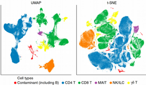
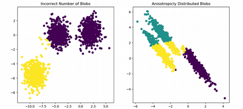
One problem with clustering scRNAseq is the discrepancy between what we see in a tSNE plot and what cluster analysis reports in terms of number of clusters and cell assignment to clusters. For example, we clearly observe three clusters in the figure below and can even manually draw boundaries between the clusters. However, running a clustering algorithm might result in artifacts such as wrong number of clusters or wrong cell assignment to clusters, i.e. when a uniform cluster happens to be split into pieces by the algorithm.

Moreover, trying to reproduce results of scientific papers might be confusing due to the lack of robustness of clustering algorithms. For example, using the data from Kolodziejczyk et al., Cell Stem Cell 2015, eight clusters are visible in the tSNE plot, however the clustering algorithm used in the paper seems to detect only three clusters.

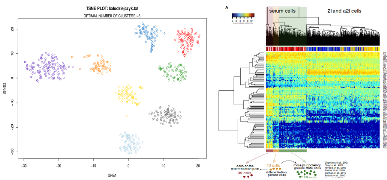
The contradiction between the dimensionality reduction and clustering has a dual nature. On the one hand, it is notoriously difficult to define a distance between data points in high-dimensional scRNAseq space due to the Curse of Dimensionality; one the other hand, clustering algorithms often use idealistic assumptions which do not hold for the real world data.

Euclidean distance breaks in High Dimensions

Mathematics of High Dimensions is an active area of research. There are many weird phenomena arising in high-dimensional space. One of them is that the distance between the data points and the origin of the coordinate system grows as a square root of the number of dimensions D. This can be seen as the data points deplete the center and concentrate in the shell of the n-dimensional ball at large D.

Consequently, the mean distance between data points diverges and looses its meaning which in turn leads to the divergence of the Euclidean distance, the most common distance used for clustering. Manhattan distance is a better choice for scRNAseq, however it does not fully help in high dimensions either.

Assumptions and limitations of clustering methods

Despite the Curse of Dimensionality is the major obstacle for cluster analysis of scRNAseq, many clustering algorithms might perform poorly even in low dimensions due to their internal assumptions and limitations. All clustering methods can roughly be divided into four groups:

1. Hierarchical clustering
2. Centroid-based clustering
3. Graph-based clustering
4. Density-based clustering

Python library Scikit-learn provides a collection of clustering methods with an excellent overview which emphasizes their advantages and disadvantages:

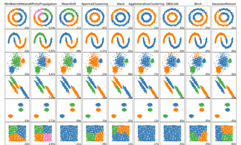
Hierarchical (agglomerative) clustering is too sensitive to noise in the data. Centroid-based clustering (K-means, Gaussian Mixture Models) can handle only clusters with spherical or ellipsoidal symmetry.

Graph-based clustering (Spectral, SNN-cliq, Seurat) is perhaps most robust for high-dimensional data as it uses the distance on a graph, e.g. the number of shared neighbors, which is more meaningful in high dimensions compared to the Euclidean distance.

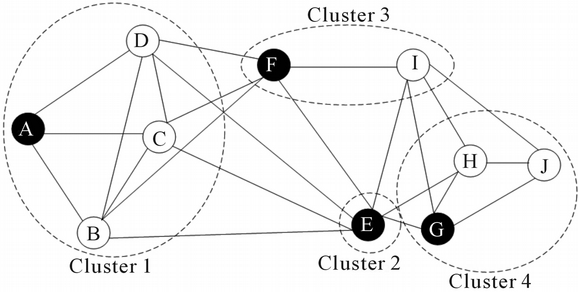
owever, to build the graph this method still uses the Euclidean distance. In addition, the number of clusters has to be implicitly specified a-priori via the “resolution” hyperparameters. Changing the hyperparameters can easily result in fewer or more clusters which is somehow arbitrary and hence quite unsatisfactory as there is no obvious way to define an objective function for automated tuning of the hyperparameters.

Out of all clustering algorithms, only Density-based (Mean-Shift, DBSCAN, OPTICS, HDBSCAN) allows clustering without specifying the number of clusters. The algorithms work via sliding windows moving toward the high density of points, i.e. they find however many dense regions are present.

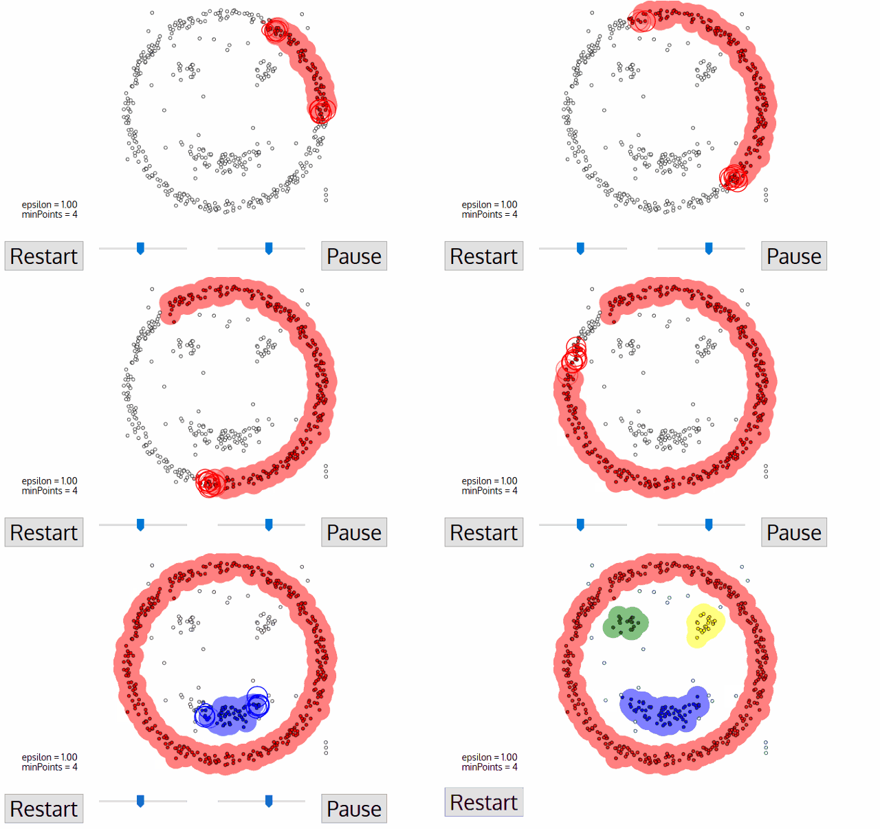
In addition, these algorithms are cluster shape independent and capture any topology of scRNAseq data. Below I will show how we can easily tune hyperparameters of the algorithm via minimization of an objective function.

How to tune hyperparameters of HDBSCAN

Clustering is an unsupervised learning problem, meaning we do not know the ground truth (number of clusters), and can not use cross-validation for optimizing hyperparameters of an algorithm. Nevertheless, there is a way to automatically optimize hyperparameters of HDBSCAN.

HDBSCAN, i.e. Hierarchical DBSCAN, is a powerful density-based clustering algorithm which is: 1) indifferent to the shape of clusters, 2) does not require the number of clusters to be specified, 3) robust with respect to clusters with different density. Further, HBDSCAN is very attractive because it has only one hyperparameter minPts which is the minimal number of points in a cluster. It is relatively fast for large data sets, detects outlying cells, and for each cell it reports a probability of assignment to a cluster. The fraction of cells with a low probability of assignment to a cluster can be used as an objective function for optimizing  minPts which in turn gives the optimal number of clusters.

Below, I will continue using the Cancer Associated Fibroblasts (CAFs) from the previous post where we found optimal perplexity (optPerp) and number of Principal Components (optPC). Now we will run HDBSCAN on the tSNE dimensionality reduction for different minimal sizes of clusters, i.e. minPts ranging from 3 to N_pt=50. For each minPts, we calculate the Score function as a fraction of cells with low confidence (probability < 5%) assignment to a cluster, by minimization of the Score function we want to reduce the number of unassigned data points. Due to internal stochasticity, tSNE changes from run to run, therefore for robustness we repeat the clustering N_iter=50 times and average the results. Plotting the Score function vs. minPts reveals a clear minimum for a certain minimal cluster size, minPts.

library("Rtsne"); library("dbscan"); library("foreach")
library("doParallel"); library("parallel")
N_iter <- 50; N_pt <- 50
score <- vector(length = N_pt-2)
for(i in 3:N_pt)
{
  score_iter <- foreach (1:N_iter, .combine = c) %dopar% 
  {
    tsne_iter <- Rtsne(t(log10(expr+1)), initial_dims=optPC,
                       perplexity=optPerp, max_iter=10000)
    res <- hdbscan(tsne_iter$Y, minPts = i)
    score_iter_temp <- sum(res$membership_prob < 0.05) / N_cells
    return(score_iter_temp)
  }
  score[i-2] <- mean(score_iter, na.rm = TRUE)
}
plot(log(score + 1) ~ seq(from=3, to=N_pt, by=1), type='o', 
     xlab="MIN SIZE OF CLUSTERS", ylab="LOG ( SCORE )")
names(score) <- seq(from=3, to=N_pt, by=1)
opt_score <- min(as.numeric(names(score)[score==min(score)]))
mtext(paste0("OPTIMAL MIN SIZE OF CLUSTERS = ",opt_score))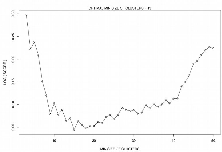

Now after we have found the optimal minimal size of clusters for our data set, minPts, we will use this value for the final HDBSCAN run on tSNE, this gives us the number of clusters, assignments of cells to the clusters, as well as cells which can not be confidently assigned to any cluster, i.e. outlying cells. The latter is an advantage and a peculiarity of density-based clustering compared to other algorithms, however here for simplicity I classified the outlying cells to their nearest neighbor clusters using the KNN classifier. Note, the tSNE was run N_tsne=50 times, and the minimal Kullback-Leibler divergence plot was selected as the final plot. Below, I show this for a few scRNAseq data sets.

library("class"); library("pals")
N_tsne <- 50
tsne_out <- list(length = N_tsne)
KL <- vector(length = N_tsne)
for(k in 1:N_tsne)
{
  tsne_out[[k]] <- Rtsne(t(log10(expr+1)),initial_dims=optPC,perplexity=optPerp,
                         max_iter=10000)
  KL[k] <- tail(tsne_out[[k]]$itercosts, 1)
}
names(KL) <- c(1:N_tsne)
opt_tsne <- tsne_out[[as.numeric(names(KL)[KL==min(KL)])]]$Y
res_opt <- hdbscan(opt_tsne, minPts = opt_score)
if(length(res_opt$cluster[res_opt$cluster==0]) > 0 & 
   length(res_opt$cluster[res_opt$cluster==1]) > 0)
{
  res_opt$cluster[res_opt$cluster==0]<-class::knn(
    opt_tsne[which(res_opt$cluster!=0),],opt_tsne[which(res_opt$cluster==0),],
    res_opt$cluster[res_opt$cluster!=0], k=3)
}
print(res_opt)
N_clust<-length(sort(unique(res_opt$cluster)))
if(N_clust <= 25){colors <- cols25(N_clust)}else{colors <- rainbow(N_clust)}
names(colors) <- sort(unique(res_opt$cluster))
plot(opt_tsne,main=paste0("TSNE PLOT: ",file_name),
     col=colors[as.character(res_opt$cluster)], xlab="tSNE1", ylab="tSNE2")
mtext(paste0("OPTIMAL NUMBER OF CLUSTERS = ", N_clust))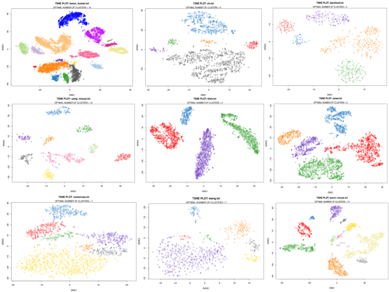

The results of applying HDBSCAN to various scRNAseq data sets do not look too bad given that these plots were obtained by providing the raw expression matrix only that is without manual tweaking of the clustering parameters.

Clustering on tSNE, PCs and raw expression matrix

Running clustering on a raw expression matrix can be very challenging due to the Curse of Dimensionality. Therefore it is almost always recommended to perform any sort of dimensionality reduction before proceeding with cluster analysis. Here I compare performance of 9 popular clustering algorithms on the CAFs data set: HDBSCAN (described above), Kmeans, Gaussian Mixture Models (GMM), Hierarchical clustering, Spectral clustering, SC3, Bootstrap Consensus Clustering, SNN-cliq and Seurat. Indeed, running the clustering algorithms on the raw CAFs expression matrix brings unsatisfactory results:

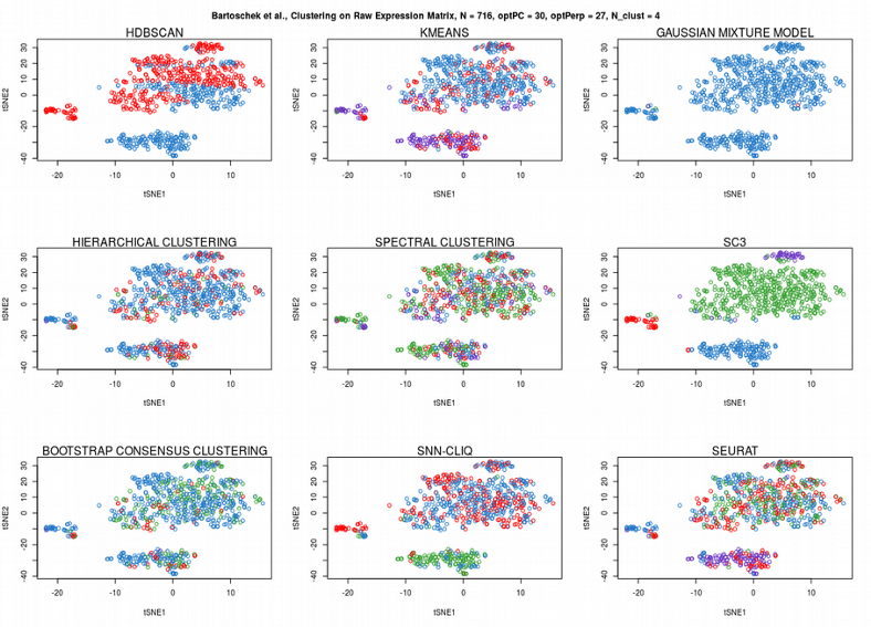
While all the algorithms fail clustering on the raw expression matrix, only SC3, which performs consensus clustering across different algorithms and distance metrics, provided surprisingly good cell assignment. Now we will apply the clustering algorithms to the significant PCs found by permuting expression matrix in the previous post.

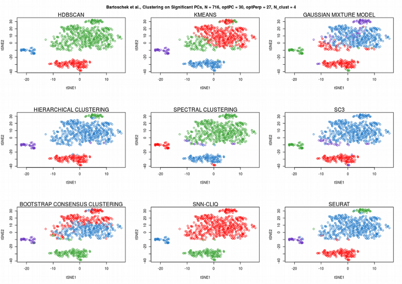
Now, SC3 did not perform so well, HDBSCAN was not perfect either. Instead, Seurat graph-based community detection and hierarchical clustering seem to perform the best. Finally, let us apply the 9 clustering algorithms to the tSNE reduced dimension representation of the scRNAseq expression data:

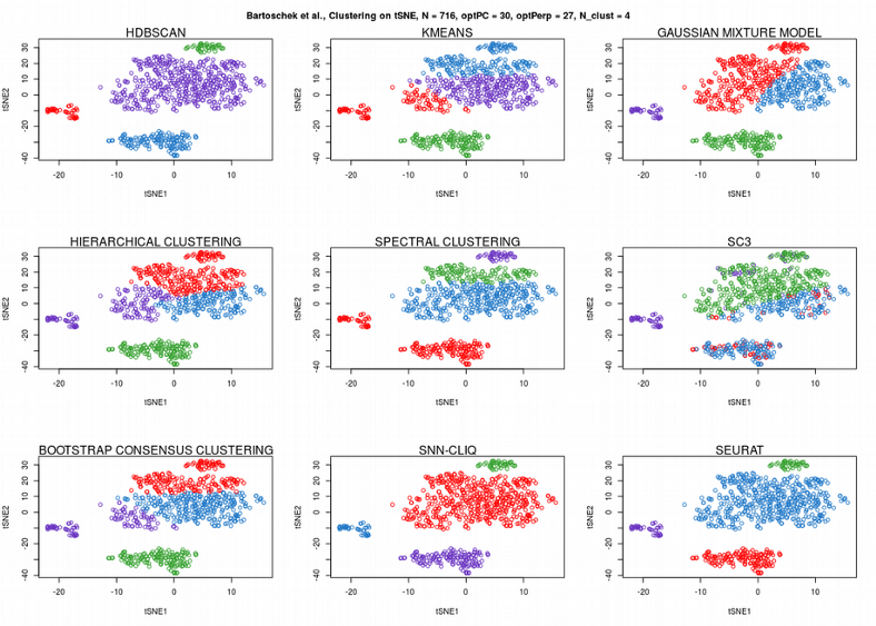
Despite tSNE plot is a 2D dimensionality reduction, many algorithms such as K-means, Gaussian Mixture Models (GMM), Hierarchical clustering, Spectral clustering, Bootsrap Consensus clustering and SC3 fail to correctly assign the cells to their clusters. HDBSCAN and graph-based clustering methods (Seurat and SNN-cliq) seem to perform the best. However, the latter needed a manual hyperparameters tweaking which was not necessary for HDBSCAN due to the automated optimization procedure described above.

Summary

In this article, we have learnt that clustering of high-dimensional scRNAseq data is challenging due to the Curse of Dimensionality and limitations of the clustering methods. Frustratingly, most of clustering algorithms require the number of clusters to be specified a-priori which is hard to optimize due to inapplicability of cross-validation for clustering. However, the HDBSCAN stands out here as an algorithm with only one hyperparameter which is easy enough to optimize via minimization of the amount of unassigned cells.gi