In my previous post, I started covering methods of removing technical variation in scRNAseq data by comparing normalization strategies. Here I am going to expand on the topic and talk about correcting systematic differences between same type of cells sequenced by different technologies, labs, protocols etc, i.e. batch-effects detection and elimination.

How to Detect Batch-Effects?

Batch-effects have a danger to confound the true biological signal, which is the discovery of the cell types present in a sample for the case of scRNAseq. Batches can originate from: different dates of sequencing, people doing the sequencing, flow-cells / plates, chemistry / protocol, lanes, read length, labs produced the data or even different organisms as the extreme case scenario.

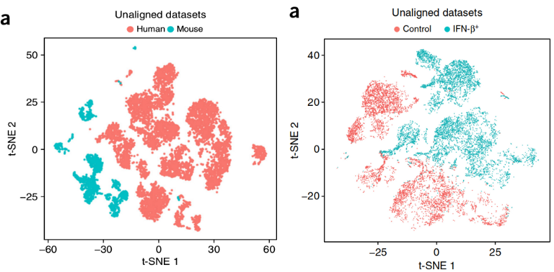
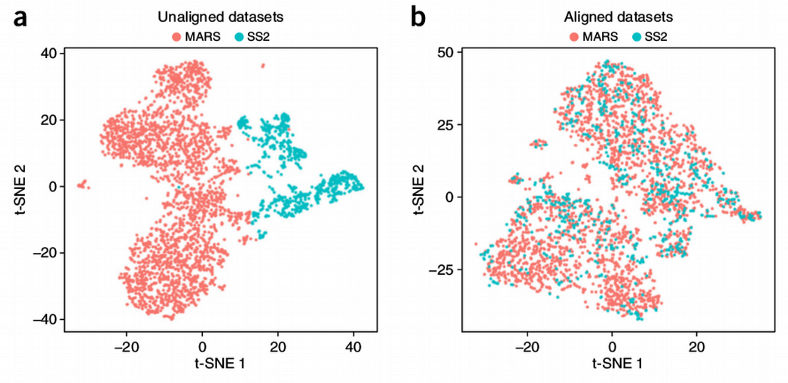
Batch-effects can be genome-wide, i.e. present for majority of genes, or gene-specific, i.e. certain genes happen to be influenced by the batch. The former is very easy to see from the dimension reduction plots like PCA or tSNE. Here for demonstration purposes I will continue using the innate lymphoid cells (ILC) scRNAseq data set from Å. Björklund et al., Nature Immunology 17, p. 451–460 (2016). Below I compute the PCA and tSNE dimensionality reduction plots for the ILC cells from three donors.

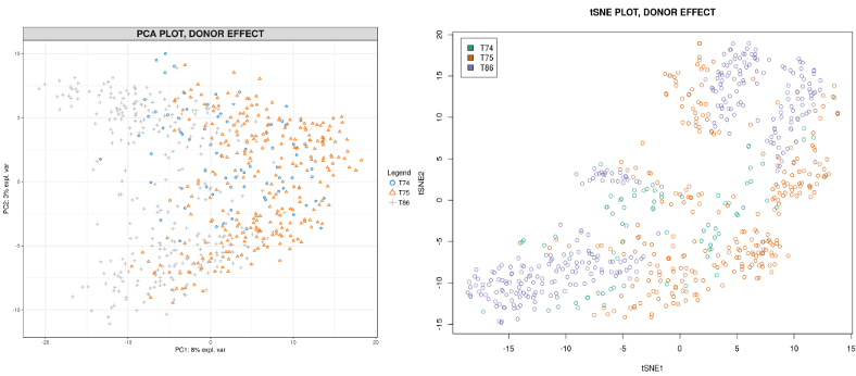
The donor-specific batch is clearly visible from the plots, i.e. the cells from the same donor tend to cluster together and distinctly from the cells coming from other donors. To further quantify, let us display how much of variation in each Principal Component (PC) is explained by the Donor, Plate and Cell Type.

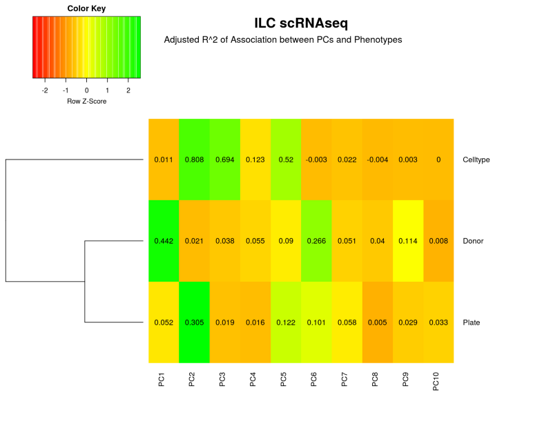
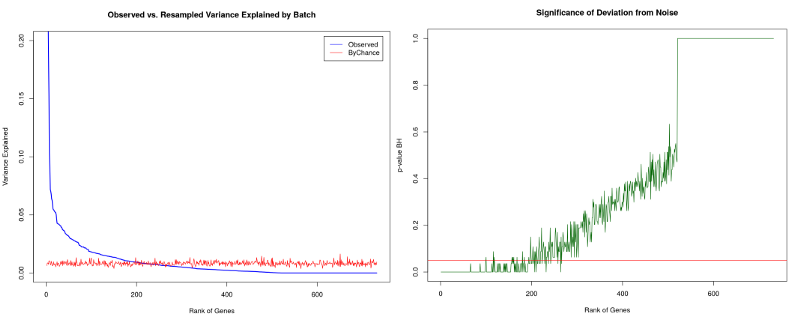
From the heatmap above it follows that 44% of PC1 is explained by the Donor batch while the Cell Type contribution is negligible, therefore we have a severe genome-wide Donor related batch effect. However, what if we did not observe any clustering by Donor at the dimension reduction plots above, does it mean that there are no batch-effects present in our data set? No it does not. Certain genes might still have their variation to a large extent due to the batch and not the cell type. We can rank all genes influenced by the batch by correlating their expression with the Donor variable. From the left figure below we observe that there aregenes with > 20% of their variation due to the Donor batch. To assess whether this number is a lot or a little we shuffle the batch variable (or alternatively the gene expression) a number of times and calculate thenoise zone, i.e. variation in gene expression due to a random variable. We can also do a formal statistical test and calculate a p-value of significance of deviation from the noise zone (right figure below). In this way, we end up with a list of approximately 200 genes which are significantly influenced by the batch, those genes are good to keep an eye on for the further downstream analysis.

How to Correct Batch-Effects?

Once we have detected the batch-effects in our data, we can apply multiple batch correction algorithms available. I do not recommend unsupervised correction similar to SVA for scRNAseq data, because scRNAseq analysis is also unsupervised with not known ground truth (cell types), thus removing the surrogate variables approximating the batch may damage the biological signal. For supervised batch correction, i.e. when the batch is known a-priori, a simple linear correction with the Combat method would be a good start.

Combat performs batch correction through the Bayesian linear regression and therefore offers a considerable improvement compared to the simple aka Frequentist linear batch removal implemented e.g. in Limma. Besides better performance for small sample sizes, Combat uses the Bayesian shrinkage towards the mean, this implies that correcting each gene we use a “mean” information from other genes while Limma does the correction gene-by-gene independently. Nevertheless, Combat applies a linear batch-effect correction.

Mutual Nearest Neighbors (MNN) algorithm uses a non-linear batch-effect correction inspired by the idea from K-Nearest Neighbors (KNN). The method tries to find most similar cells (mutual neighbors) between the batches, those cells are assumed to belong to the same type and the systematic differences between the MNN cells quantify the strength of the batch, this information is used to scale the rest of the cells in the batches.

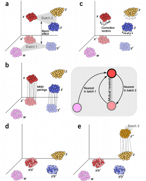
My general problem with this method is that I always failed to understand the assumption that the MNN cells should belong to the same type. My intuition is that a batch can completely mess up the concept of distance between the cells in the batches, so two cells that are closest neighbors between the batches can actually belong to different cell types but seem to be very similar because of the batch itself. Nevertheless, the MNN batch-effect correction seems to work well in practice and we will see later that it does a good job on our benchmark.

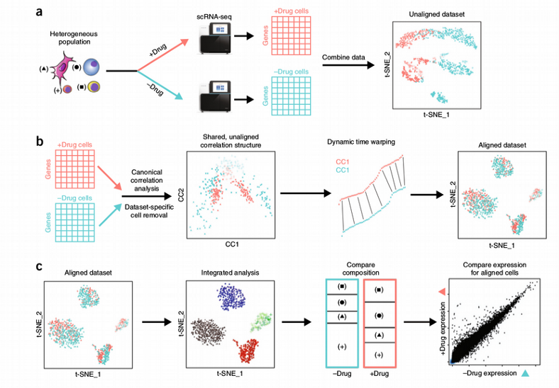
Another popular scRNAseq specific batch correction method which sometimes is seen as an across samples integration is the Seurat Canonical Correlation Analysis (CCA) technique. The concept of CCA is very similar to the PLS data integration which I described in one of my previous posts. The data from the batches are projected into a low-dimensional space by maximizing correlation (or covariance) between the data sets from different batches. This implies that the projections of the data sets are correlated but not necessarily aligned, i.e. do not overlap quite well in the low-dimensional space. The latter is solved by applying the Dynamic Time Warping (DTW) technique that locally stretches and squeezes the CCA data projections in order to further align them.

While Combat, MNN and Seurat CCA seek to transform the data in order to merge the sub-sets from different batches, SCMAP algorithm tries to project the query cells onto a reference data set, that might be e.g. the Human Cell Atlas, without actually producing a single corrected data set.

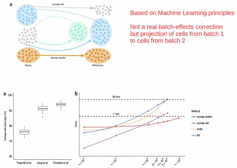
SCMAP uses a KNN classifier for finding correspondence between tested cells and a presumably much bigger reference data set which was used for training the classifier.

SCMAP uses a KNN classifier for finding correspondence between tested cells and a presumably much bigger reference data set which was used for training the classifier.

Comparing Batch Correction Methods for ILC

How do these methods work in practice? We will use the ILC scRNAseq data set in order to run them and try to remove the Donor related batch effect and thus harmonize the cells between the batches. Skipping the technicalities, here are the final comparison of tSNE plots:

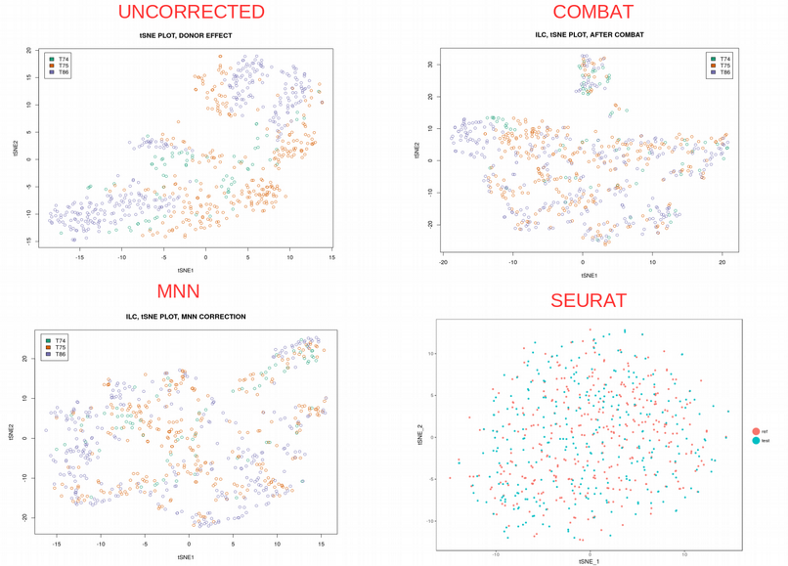
Looking at the tSNE plots above, I would say that all the methods have done a good job by well mixing the cells from different donors. Following the Occam’s Razor principle, I think the performance of the simplest Combat is satisfactory enough while being super easy to understand and program.

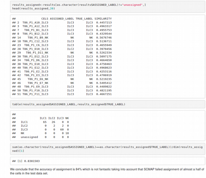
Interestingly, when training the SCMAP classifier on two donors as a reference and projecting the cells from the third donor on the the reference resulted in a poor cell assignment / classification accuracy of 84% taking into account that about the half of the cells could not be reliably assigned to any cluster at all. This might be due to the training set was not big enough or the data did not satisfy the spherical symmetry that is crucial for the KNN classifier.

Summary

In this post, we have learnt that batch-effects represent a technical variation which might confound the biological signal in scRNaseq analyses. These effects can be detected in genome-wide or gene-specific way and corrected using linear (Combat) or non-linear (MNN, Seurat CCA, SCMAP) algorithms. Overall, the batch correction methods work well on benchmarks suggesting that the simplest (Combat) model should be prioritized.