In this post I will demonstrate how analytical modelling fails reconstructing true relations between variables when increasing dimensionality of the data.

Multivariate Analysis in High Dimensions

Consider a simple linear model $Y \sim X$, where $Y$ is the response and $X$ is the explanatory (predictor) variable. $Y$ can be a phenotype vector, e.g. disease status (sick / healthy) for each of n individuals / samples, while $X$ is a matrix with $n$ samples and $p$ features / dimensions. For simplicity, both $X$ and $Y$ are drawn from normal distribution. Assume low dimensional case $ n >> p $:

set.seed(123)
n <- 20             # number of samples 
p <- 2              # number of features / dimensions 
Y <- rnorm(n)
X <- matrix(rnorm(n*p), n, p)
summary(lm(Y~X))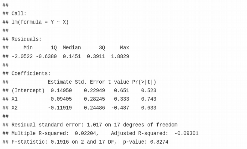

The result looks good, $Y$ and $X$ variables are not related as expected since they are drawn from the normal distribution. The math works without problems as long as $n > p$. Let us now increase the number of features / dimensions $p$ and see what happens.

set.seed(123456)
n <- 20
p <- 20
Y <- rnorm(n)
X <- matrix(rnorm(n*p),n,p)
summary(lm(Y~X))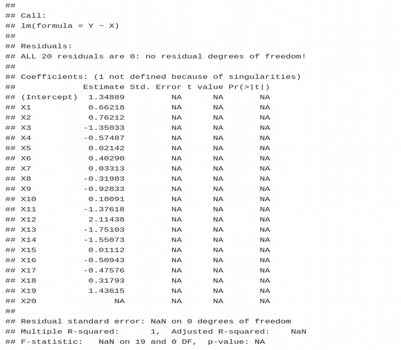

Intriguing! R refuses calculating multivariate linear model when $p = n$ despite we have only 20 dimensions. The effect we observe here is called overfitting which can be thought as one manifestation of the Curse of Dimensionality. Overfitting implies that we can not use as many fitting parameters as we want but should select their optimal number based on some additional criterion, e.g. Akaike Information Criterion (AIC), or perform the cross-validation as the number of predictors is essentially a hyperparameter of the multivariate linear model.

So we had R throwing a “singularity” error for just 20 dimensions, in fact we typically have tens of thousands (RNAseq) and even millions (genomics, methylation) dimensions in computational biology with only n=100–1000 samples. This is the main obstacle for multivariate analysis in Life Sciences and one reason why the univariate feature selection (association studies, differential gene expression, differential methylation) is often preferred over the multivariate feature selection despite the higher predictive power of the latter. Another consequence of the typical biological setup, $n << p$, is the necessity to pre-select informative features with Lasso/Ridge/Elastic Net and perform dimensionality reduction.

Adjusting for Covariates Hides True Effects

Now imagine that $X$ is not a matrix but vector, for example a genotype vector, so we are performing an association study phenotype $Y$ vs. genotype $X$. Often I observe attempts to account for additional factors (covariates) which might confound this association. Indeed, if individuals come from different human populations such as African, European, Asian, this heterogeneity may explain a significant percent of variation in the phenotype $Y$ while we are interested in the phenotypic variation explained by the genotypes, in other words the population heterogeneity is a confounding factor which should be adjusted for in the model $Y \sim X$. Typically, the Principal Component Analysis (PCA) is performed on all available genetic variants and a handful of $PCs$ is selected as covariates for the association:

\[ Y \sim X + PC_{1} + PC_{2} + …+ PC_{n} \]

In this case the number of covariates is selected somehow arbitrary based on common sense, while here I would like to demonstrate that this number might be crucial for recovering true effects of phenotype vs. genotype associations.

Let us simulate a linear relation between $X$ and $Y$ as:

\[ Y=2*X + N(\mu, \sigma) \],

where $N(\mu, \sigma)$ is a noise distribution. Suppose we have a linear model $Y \sim X$, let us adjust this model for gradually increasing number of PCs slightly correlated with $Y$, i.e. \(PC_{1}=0.9*Y\); \(PC_{2}=0.8*Y\) etc.:

set.seed(12345)

# Simulate data y~x with true effect 2 of x
N <- 100
x <- rnorm(N)
y <- 2 * x + rnorm(N)
df <- data.frame(x, y)

# Add PCs to the linear model
for (i in 1:10) {
  df[, paste0("PC", i)] <- 1 * (1 - i / 10) * y + rnorm(N)
}

# Perform linear regression gradually increasing dimensionality
effect <- vector()
effect <- append(effect, 2)
adj_r_squared <- vector()
adj_r_squared <- append(adj_r_squared, summary(lm(y ~ x, data = df))$adj.r.squared)

for (i in 1:10) {
  formula <- as.formula(paste0("y~x+", paste0("PC", seq(1:i), collapse = "+")))
  effect <- append(effect, summary(lm(formula, data = df))$coefficients[2, 1])
  adj_r_squared <- append(adj_r_squared, summary(lm(formula, data = df))$adj.r.squared)
}

plot(effect ~ seq(from = 0, to = 10, by = 1), type = 'o',
     xlab = "PRINCIPAL COMPONENTS", ylab = "EFFECT")
plot(adj_r_squared ~ seq(from = 0, to = 10, by = 1), type = 'o',
     xlab = "PRINCIPAL COMPONENTS", ylab = "VARIANCE EXPLAINED BY MODEL")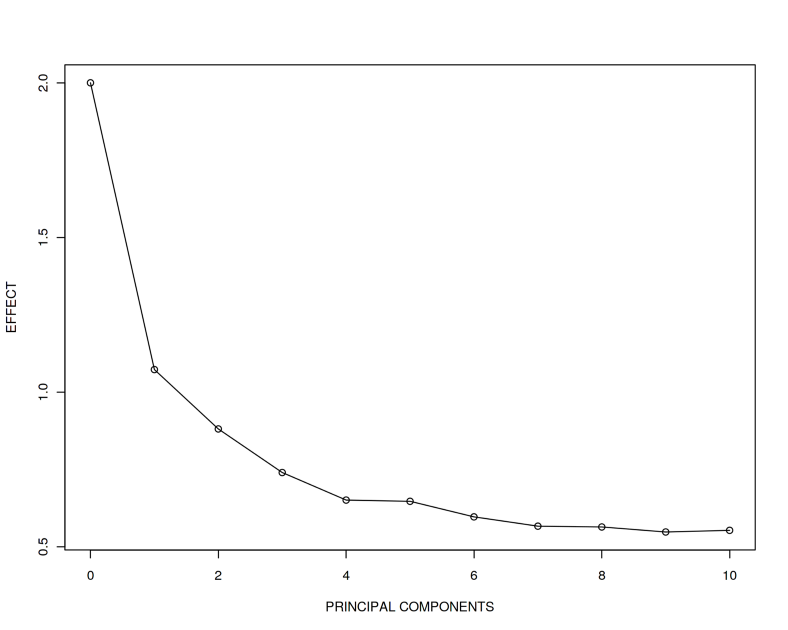

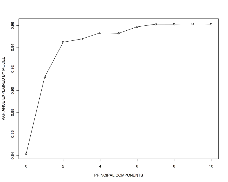
What we observe here is that the true effect 2 of association between $Y$ and $X$ becomes more and more difficult to recover when adding $PCs$ correlated with $Y$. Despite we still have $n > p$, when 10 $PCs$ are added, the recovered effect is approximately 0.5 which is far from the true effect 2. In addition, we observe that the adjusted R squared (variance explained) reaches almost 1 implying we explain essentially all the variance in $Y$ by including only 10 covariates.

In the code above please note the coefficient 1 in front of (1-$i$/10). Let us call this a covariation coefficient between $Y$ and $PCs$. We have just seen that for the case when $Covariation=1$, the true effect 2 can be falsely calculated as 0.5. What happens now if we increase the covariation between $Y$ and $PCs$, i.e. for $Covariation=2$ and $3$?

effect_master <- list()

for (k in 1:3) {
  for (i in 1:10) {
    df[, paste0("PC", i)] <- k * (1 - i / 10) * y + rnorm(N)
  }

  effect <- vector()
  effect <- append(effect, 2)
  for (i in 1:10) {
    formula <- as.formula(paste0("y~x+", paste0("PC", seq(1:i), collapse = "+")))
    effect <- append(effect, summary(lm(formula, data = df))$coefficients[2, 1])
  }
  effect_master[[k]] <- effect
}

plot(effect_master[[1]] ~ seq(from = 0, to = 10, by = 1), type = 'o',
     xlab = "PRINCIPAL COMPONENTS", ylab = "EFFECT", xlim = c(0, 10), ylim = c(0, 2), col = "blue",
     main = "Effect of x vs. y at different covariation between y and PCs")

points(effect_master[[2]] ~ seq(from = 0, to = 10, by = 1), col = "green")
lines(effect_master[[2]] ~ seq(from = 0, to = 10, by = 1), col = "green")
points(effect_master[[3]] ~ seq(from = 0, to = 10, by = 1), col = "red")
lines(effect_master[[3]] ~ seq(from = 0, to = 10, by = 1), col = "red")
legend("topright", c("1", "2", "3"), title = "Covariation", fill = c("blue", "green", "red"),
       inset = 0.02)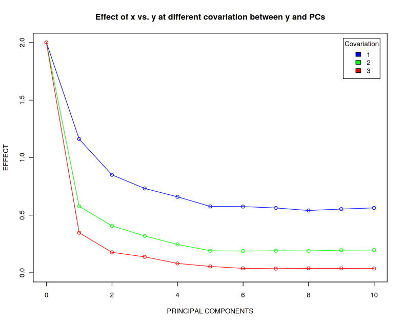

We observe that the more $Y$ is correlated with the covariates $PCs$, the harder it is to reconstruct the true effect. When $Covariation=3$, the reconstructed effect is essentially zero which implies that there is no association between $Y$ and $X$ despite we have simulated this effect to be 2. Therefore, even though it can make a lot of biological sense to adjust your linear model for covariates, this should be performed with caution since the math might not stand it due to the Curse of Dimensionality.

Summary

In this article, we have learnt that multivariate analysis blows up when the number of features / dimensions approaches the number of samples due to the Curse of Dimensionality. In addition, performing association studies you should pay particular attention to the number of covariates your linear model is adjusted for. Too many covariates might blur the true effects and make their reconstruction impossible.