Here we are going to talk about dimension reduction techniques applied to single cell genomics data. Among others, we are going to compare linear and non-linear dimension reduction techniques in order to understand why tSNE and UMAP became golden standard for Single Cell biology.

Non-Linear Structure of Single Cell Data

Single cell genomics is a high dimensional data with approximately 20 000 dimensions corresponding to the protein coding genes. Usually not all of the genes are equally important for the cellular function, i.e. there are redundant genes which can be eliminated from the analysis in order to simplify the data complexity and overcome the Curse of Dimensionality. To exclude redundant genes and project the data onto a latent space where the hidden stricture of the data becomes transparent is the goal of dimension reduction.

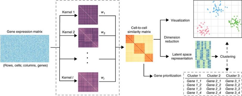
Principal Component Analysis (PCA) is a basic linear dimension reduction technique which has been widely recognized to be inappropriate for the single cell data due to their highly non-linear structure. Intuitively the non-linearity comes from the large fraction of stochastic zeros in the expression matrix due to the dropout effect. Typically, single cell data have 60–80% zero elements in the expression matrix. In this way, single cell data are similar to image data where e.g. for the images of hand-written digits MNIST data set we have 86% of pixels having zero intensity.

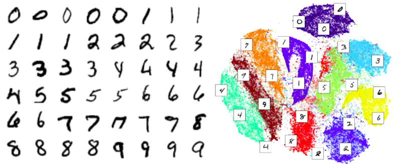
This large percentage of stochastic zeros in the expression matrix makes the data behave similar to the non-linear Heaviside step function, i.e. the gene expression is either zero or non-zero regardless of how much “non-zero”. Let us demonstrate basic linear and non-linear dimension reduction techniques applied to the Cancer Associated Fibroblasts (CAFs) single cell data set.

Linear Dimension Reduction Techniques

We are going to start with the linear dimension reduction techniques. Here we read and log-transform the single cell CAFs expression data, the latter can be viewed as a way to normalize the data. As usually, the columns are genes and the rows are cells, the last column corresponds to the IDs of the 4 populations (clusters) found previously in the CAFs data set.

import numpy as np
import pandas as pd
expr = pd.read_csv('CAFs.txt',sep='\t')
print("\n" + "Dimensions of input file: " + str(expr.shape) + "\n")
print("\n" + "Last column corresponds to cluster assignments: " + "\n")
print(expr.iloc[0:4, (expr.shape[1]-4):expr.shape[1]])
X = expr.values[:,0:(expr.shape[1]-1)]
Y = expr.values[:,expr.shape[1]-1]
X = np.log(X + 1)

Now we are going to apply the most popular linear dimensionality reduction techniques using the scikit-learn manifold learning library. Check here for the complete script, here for simplicity I show only the codes for the Linear Discriminant Analysis (LDA):

from sklearn.discriminant_analysis import LinearDiscriminantAnalysis

model = LinearDiscriminantAnalysis(n_components = 2, priors = None,
                                   shrinkage = 'auto', 
                                   solver = 'eigen',
                                   store_covariance = False,
                                   tol = 0.0001)

lda = model.fit_transform(X, Y)

plt.scatter(lda[:, 0], lda[:, 1], c = Y, cmap = 'viridis', s = 1)
plt.xlabel("LDA1", fontsize = 20); plt.ylabel("LDA2", fontsize = 20)
feature_importances = pd.DataFrame({'Gene':np.array(expr.columns)[:-1], 
                                    'Score':abs(model.coef_[0])})
print(feature_importances.sort_values('Score', ascending = False).head(20))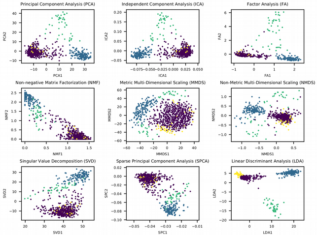

What we can immediately conclude is that the linear dimensionality reduction techniques can not fully resolve the heterogeneity in the single cell data. For instance, the small yellow cluster does not seem to be distinct from the other 3 cell clusters. The only exception is the LDA plot, however this is not a truly unsupervised learning method as in contrast to the rest it uses the cell labels in order to construct the latent features where the classes are most separable from each other. Thus the linear dimension reduction techniques are good at preserving the global structure of the data (connections between all the data points) while it seems that for single cell data it is more important to keep the local structure of the data (connections between neighboring points).

It is really fascinating to observe how the data is converted into the latent low-dimensional representation, and each of the dimension reduction techniques deserves its own article. It is interesting to think about why basically each of the techniques is applicable in one particular research area and not common in other areas. For example, Independent Component Analysis (ICA) is used in signal processing, Non-Negative Matrix Factorization (NMF) is popular for text mining, Non-Metric Multi-Dimensional Scaling (NMDS) is very common in Metagenomics analysis etc., but it is rare to see e.g. NMF to be used for RNA sequencing data analysis.

Non-Linear Dimension Reduction Techniques

We turn to the non-linear dimension reduction techniques and check whether they are capable of resolving all hidden structure in the single cell data. Again, complete codes can be found here, for simplicity I show below only the code for the tSNE algorithm which is known to have difficulty handling really high dimensional data and hence is common to be run on 20–50 pre-reduced dimensions with e.g. PCA.

from sklearn.manifold import TSNE
from sklearn.decomposition import PCA
X_reduced = PCA(n_components = 30).fit_transform(X)
model = TSNE(learning_rate = 10, n_components = 2, random_state = 123, perplexity = 30)
tsne = model.fit_transform(X_reduced)
plt.scatter(tsne[:, 0], tsne[:, 1], c = Y, cmap = 'viridis', s = 1)
plt.title('tSNE on PCA', fontsize = 20)
plt.xlabel("tSNE1", fontsize = 20)
plt.ylabel("tSNE2", fontsize = 20)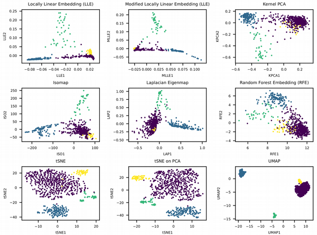

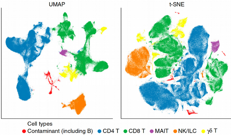
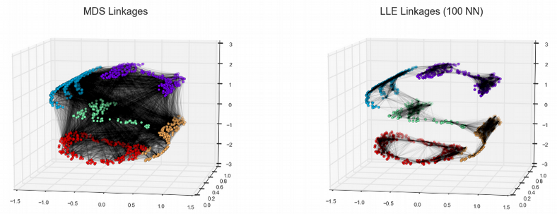
Here we see that most of the non-linear dimensionality reduction techniques have successfully resolved the small yellow cluster via preserving the local structure (connections between neighboring points) of the data. For instance, the Locally Linear Embedding (LLE) approximates the non-linear manifold by a collection of locally linear planar surfaces which happens to be crucial for reconstructing the rare cell populations such as the small yellow cluster. The best visualization though comes from tSNE and UMAP. The former captures the local structure as well as LLE, and seems to work on raw expression data in this particular case, however a pre-dimension reduction with PCA provides typically more condensed and distinct clusters. In contrast, UMAP preserves both the local and the global data structure and is based on the topological data analysis where a manifold is represented as a collection of elementary Simplex units, this ensures that the distances between the data points do not look all equal in the high-dimensional manifold but there is a distribution of distances similar to the 2D space. In other words, UMAP is an elegant attempt to beat the Curse of Dimensionality.

Summary

In this post, we have learnt that single cell genomics data have a non-linear structure which comes from the large proportion of stochastic zeros in the expression matrix due to the drop out effect. The linear manifold learning techniques preserve the global structure of the data and are not capable of fully resolving all cell populations present. In contrast, preserving the local connectivity between the data points (LLE, tSNE, UMAP) is the key factor for a successful dimensionality reduction of single cell genomics data.