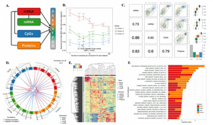
In the previous post I introduced the topic and explained why we need to do feature selection before proceeding with the integration. Here I will explain how to perform supervised OMICs integration using Partial Least Square (PLS) regression and Discriminant Analysis.

Chronic Lymphocytic Leukemia (CLL) Data Set

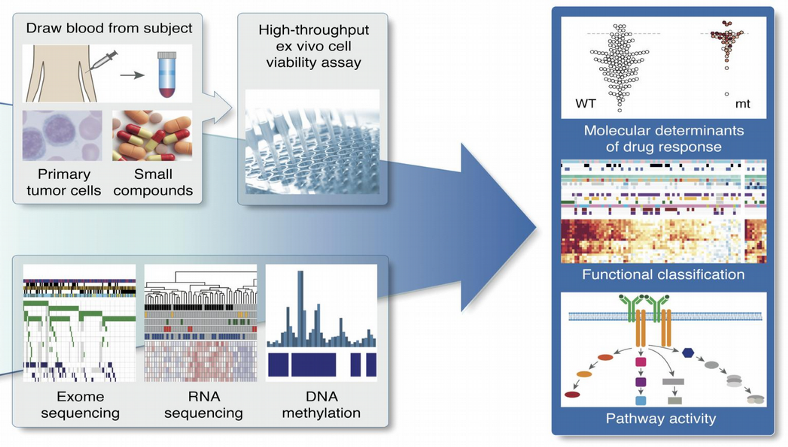
Integration of multiple molecular OMICs represents a contemporary challenge in computational Biology and Biomedicine as Big Data becomes a reality here. One example of biomedical data with multiple OMICs which we will use here is the study of Chronic Lymphocytic Leukemia (CLL). This study combined drug response with somatic mutation information, transcriptome profiling and DNA methylation assays.

Traditional biological approach to perform integration has been for decades the pair-wise correlations of OMICs layers. Despite its interpretability and simplicity this approach was recognized to provide inconsistent information for the case of multiple OMICs sets. To overcome the problem of technological dissimilarities between different data sets, a more promising idea of OMICs integration is to represent each data set by latent variables which contain no memory of the technology they were produced by.

PLS-DA Integration with DIABLO

The most straightforward implementation of the idea of latent variables is the multivariate integration of multiple OMICs based on the Partial Least Squares (PLS) regression and discriminant analysis when most informative features from different OMICs are being selected with the constraint of correlation between their first PLS components. This method has become very popular due to its simplicity and efficient implementation in the R package mixOmics.

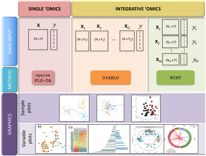
MixOmics includes several elegant statistical algorithms, among others MINT represent across samples integration, similar to batch effect correction, and DIABLO represents across OMICs integration, which is the true multi-OMICs data integration which we are going to use here for the CLL data set.

CLL OMICs Integration with DIABLO

We will start with reading the CLL data and imputing the missing values with the simple median imputation. We will use Gender as the trait of interest, thus PLS-DA algorithm will perform extraction of features simultaneously across multiple OMICs that maximize the separation between Males and Females in the low-dimensional latent PLS space. Since we direct the feature extraction with the Gender variable, this is a supervised OMICs integration method.

expr <- as.data.frame(t(read.delim("CLL_mRNA.txt", header = TRUE, sep = "\t")))
for (i in 1:ncol(expr)){
    expr[, i][is.na(expr[, i])] <- median(expr[, i], na.rm = TRUE)
}

mut <- as.data.frame(t(read.delim("CLL_Mutations.txt", header = TRUE, sep = "\t")))
for (i in 1:ncol(mut)){
    mut[, i][is.na(mut[, i])] <- median(mut[, i], na.rm = TRUE)
}

meth <- as.data.frame(t(read.delim("CLL_Methylation.txt", header = TRUE, sep = "\t")))
for (i in 1:ncol(meth) 
    meth[, i][is.na(meth[, i])] <- median(meth[, i], na.rm = TRUE)
}

drug <- as.data.frame(t(read.delim("CLL_Drugs.txt", header = TRUE, sep = "\t")))
for (i in 1:ncol(drug)
    drug[, i][is.na(drug[, i])] <- median(drug[, i], na.rm = TRUE)
}

phen <- read.delim("CLL_Covariates.txt", header = TRUE, sep = "\t")
Y <- factor(phen$Gender)

Next we will split the n=200 CLL samples into train (n=140) and test (n=60) data sets for later testing the model for prediction accuracy. Since mutations represent a binary data, there is always a lack of variation due to coding with 0 and 1. Therefore, we will pre-filter the mutation matrix by excluding the sites with variance across individuals close to zero. Next, since gene expression and methylation data sets are high-dimensional, we use LASSO to perform feature pre-selection in the way I described in the previous post. Next, we perform cross-validation for selecting the optimal number of predictive components:

library("mixOmics")

data <- list(expr = expr, mut = mut, meth = meth, drug = drug)
design <- matrix(1, ncol = length(data), nrow = length(data), dimnames = list(names(data), names(data)))
diag(design) <- 0

splsda.res <- block.splsda(X = data, Y = Y, ncomp = 8, design = design)
perf.diablo <- perf(splsda.res, validation = 'Mfold'
                    folds = 2, nrepeat = 5,
                    progressBar = FALSE, cpus = 4)
plot(perf.diablo, overlay = 'dist', sd = TRUE)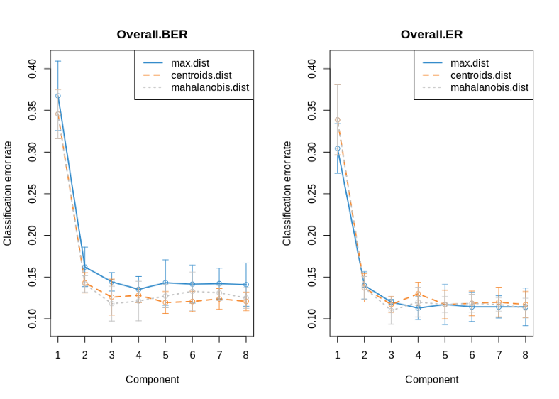

The classification error rate seems to reach its plateau at ncomp=2, so we will use this number as an optimal number of predictive components to keep in the further downstream analysis. The design matrix above defines the expected covariance between the OMICs. Here due to the lack of prior knowledge we select a strong correlation 1 between the OMICs. Further, we again will use cross-validation in order to determine the optimal number of features for each OMIC to be used for extracting most predictive variables with LASSO when running the sparse PLS-DA. Finally, after we have found the optimal numbers of predictive components and variables in each OMIC, we run the sparse PLS-DA for OMICs integration.

test.keepX <- list("expr" = c(1:5), "mut" = c(1:5), "meth" = c(1:5), "drug" = c(1:5))
tune.omics <- tune.block.splsda(X = data, Y = Y, ncomp = 2, test.keepX = test.keepX,
                                design = design, cpus = 4, validation = "Mfold",
                                folds = 2, nrepeat = 5, dist = "mahalanobis.dist")
                             
list.keepX <- list("expr" = tune.omics$choice.keepX$expr, "mut" = c(dim(mut)[2], dim(mut)[2]),
                   "meth" = tune.omics$choice.keepX$meth, "drug" = tune.omics$choice.keepX$drug)

res <- block.splsda(X = data, Y = Y, ncomp = 2, keepX = list.keepX,
                    design = design, near.zero.var = FALSE)
                    
plotIndiv(res, legend = TRUE, title = "CLL Omics", ellipse = FALSE, ind.names = FALSE, cex = 2)
plotArrow(res, ind.names = FALSE, legend = TRUE, title = "CLL Omics Integration")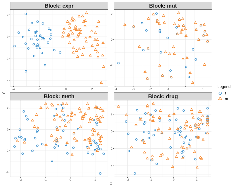

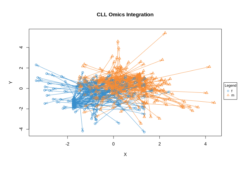
The quartet of plots above shows the low-dimensional PLS representation of individual OMICs after integrative feature extraction has been performed. In contrast, the so-called Arrow Plot below can be thought as a consensus plot across the OMICs. It demonstrates quite clear separation between Males and Females due to simultaneous across OMICs features extraction with PLS-DA.

Biological Intepretation of Integration Results

MixOmics provides lots of impressive visualization for biological interpretation of the data. Here we present the Correlation Circle Plot, where the variables from the top loadings from each of the OMICs are superimposed. Clustering of the variables around the poles of the circle implies strong correlation between the variables from the OMICs data sets. Variables on the opposite poles of the correlation circle plot imply strong anti-correlation.

plotVar(res, var.names = TRUE, style = 'graphics', legend = TRUE, pch = c(16, 17, 18, 19),
        cex = c(0.8, 0.8, 0.8, 0.8), col = c('blue', 'red2', "darkgreen", "darkorange"))

circosPlot(res, cutoff = 0.7, line = FALSE, size.variables = 0.5)
network(res, blocks = c(1, 2), cex.node.name = 0.6, color.node = c('blue', 'red2'))
network(res, blocks = c(1, 3), cex.node.name = 0.6, color.node = c('blue', 'darkgreen'))
network(res, blocks = c(1, 4), cex.node.name = 0.6, color.node = c('blue', 'darkorange'))
network(res, blocks = c(2, 3), cex.node.name = 0.6, color.node = c('red2', 'darkgreen'))
network(res, blocks = c(2, 4), cex.node.name = 0.6, color.node = c('red2', 'darkorange'))
network(res, blocks = c(3, 4), cex.node.name = 0.6, color.node = c('darkgreen', 'darkorange'))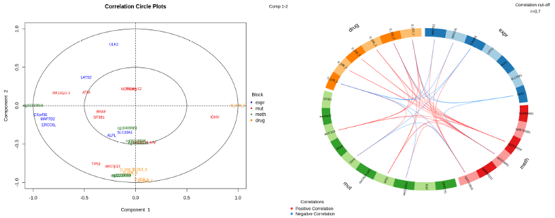

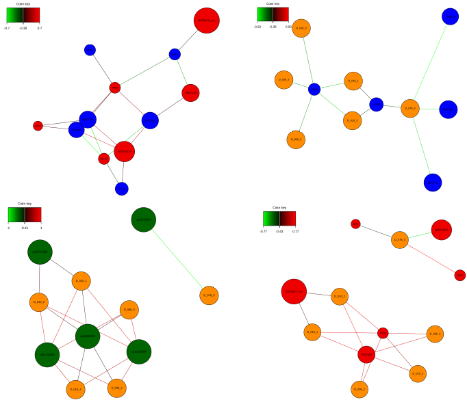
Another way to present correlations between most informative features across the OMICs is the so-called Circos Plot. Again, the variables for this plot were selected simultaneously from all the OMICs, i.e. they are different from those obtained from each individual OMIC separately. Correlation Network is yet another way to demonstrate correlations between most informative features across the OMICs data sets in a pairwise fashion.

Prediction with DIABLO Integrative Model

Now it is time for prediction. Once we have trained the PLS-DA model, we can use it and utilize the 60 test samples for making prediction of their gender and accessing the accuracy of the prediction:

data.test <- list(expr = expr_test, mut = mut_test, meth = meth_test, drug = drug_test)
predict.diablo <- predict(res, newdata = data.test, dist = 'mahalanobis.dist')
auroc.diablo <- auroc(res, newdata = data.test, outcome.test = Y.test, plot = TRUE,
                      roc.comp = c(1), roc.block = c(1, 2, 3, 4))

data.frame(predict.diablo$class, Truth = Y.test)
table(predict.diablo$MajorityVote$mahalanobis.dist[, 1], Y.test)
round((sum(diag(table(predict.diablo$MajorityVote$mahalanobis.dist[, 1], Y.test)))
       / sum(table(predict.diablo$MajorityVote$mahalanobis.dist[, 1], Y.test))) * 100)

Typically the success rate (accuracy) of predicting the gender from the DIABLO integrative model on the CLL data set is 60–70% which is not fantastic since it is a linear integration method. We can do it better with non-linear integration model via artificial neural networks which I will explain in the next posts.

Summary

In this post, we have learnt that PLS-DA is an elegant multivariate method for OMICs integration which projects individual data sets on a common latent low-dimensional space where the data sets loose the memory of their initial technological differences. The OMICs can be merged in this common latent space and the trait classes (aka sick-healthy) become linearly separable.