Previously, I gave an introduction to OMICs integration and covered the supervised PLS-DA model. Today we will consider unsupervised OMICs integration which is especially handy when no class labels (no clear phenotypes) are available, but we still would like to understand heterogeneity between the samples in our data by combining different sources of biological information.

Supervised vs Unsupervised Data Integration

To compare supervised and unsupervised data analyses is like comparing The Beatles and The Velvet Underground music. Both are excellent but in different ways. While supervised modeling dominates in the modern research since it provides slow but guaranteed progress, unsupervised models have always been considered as a “high risk - high gain” approach.

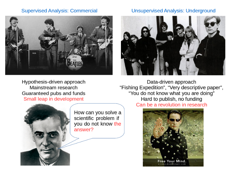
The question of Lev Landau (Nobel Prize winner in Physics) which he asked his students struggling to solve mathematical problems: “How can you solve a scientific problem without knowing the answer?” reflects the mentality of supervised hypothesis-driven mainstream research. For instance, if one dares to reply “I do not have any” to the editor’s comment “I do not quite understand your biological hypothesis”, this will most likely lead to a rejection of the paper from a peer-review scientific journal. This is because in the research we tend to constrain ourselves with an initial idea of how the things work and the study to be done is just to prove our hypothesis is true. In contrast, the unsupervised approach is a free your mind approach when you have no idea about what is in your data and therefore open to discovering unexpected phenomena.

Multi-OMICs Factor Analysis (MOFA)

MOFA is a typical hypothesis-free data exploration framework. It allows data integration by extracting common axes of variation from the multiple OMICs layers. Given data matrices from multiple OMICs on the same or overlapping samples, MOFA infers a low-dimensional representation of the data in terms of latent / hidden factors which can be then visualized and interpreted.

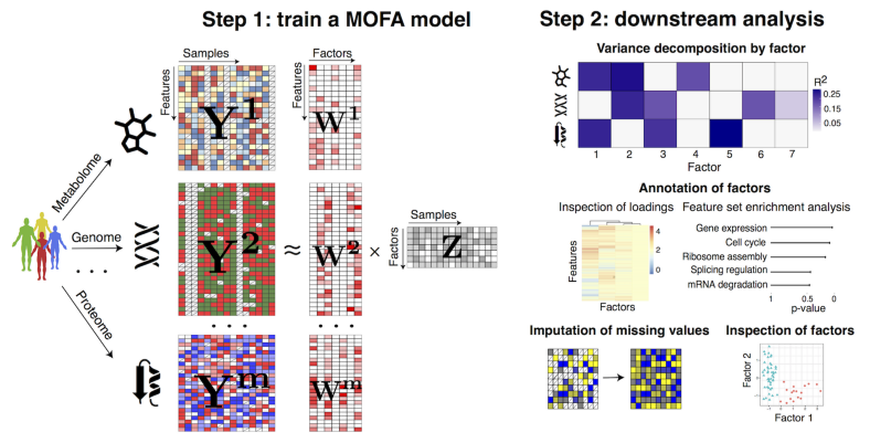
Similar to other integrative OMICs methods such as DISCO, JIVE and O2PLS, MOFA infers if the underlying axes of heterogeneity are unique to individual OMIC or manifested in multiple OMICs. In addition, MOFA provides several useful features including:

• Visualization of samples in low-dimensional latent space
• Annotation of factors using (gene set) enrichment analysis
• Imputation and support of missing and sparse data
• Support of OMICs with non-Gaussian distributions

The latter two advantages originate from the fact that MOFA is implemented within the Bayesian framework which does not depend on the assumptions of Frequentist statistics such as large amount of data or Gaussian distribution. Importantly, MOFA is a linear integrative OMICs algorithm, a more general non-linear OMICs integration can be performed via e.g. autoencoders. Final remark to mention about MOFA is that it is a Factor Analysis (FA) algorithm, and despite FA visually might look identical to PCA, those two linear dimension reduction techniques should not be confused. While PCA is a pure matrix factorization technique (unless it is a Probabilistic PCA) which splits the total variance into orthogonal Principal Components, FA seeks to construct hidden latent variables that generate the observed data, therefore Factor Analysis is a generative model similar to the Hidden Markov Model (HMM), Gaussian Mixture Models (GMM), Variational Autoencoder (VE), Generative Adversarial Networks (GANs) etc.

Integration of scNMT Multi-OMICs Data Set

In this section, we will apply MOFA to the single cell multi-OMICs scNMT data set which profiles chromatine accessebility (scATACseq), DNA methylation (scBSseq) and gene expression (scRNAseq) from the same biological cells belonging to two types: differentiating mouse embryonic stem cells (ESCs) and embrionic bodies (EBs). We will start with reading and filtering and log-transforming the scRNAseq subset of scNMT:

scRNAseq <- read.delim("scRNAseq.txt", header = TRUE, check.names = FALSE, row.names = 1, sep = "\t")
ens2genesymbol <- read.delim("ENSEMBLE_TO_GENE_SYMBOL_MOUSE.txt")
ens2genesymbol <- ens2genesymbol[match(colnames(scRNAseq), as.character(ens2genesymbol$ensembl_gene_id)),]
colnames(scRNAseq) <- ens2genesymbol$external_gene_name
scRNAseq <- as.data.frame(t(scRNAseq))
scRNAseq <- scRNAseq[rowMeans(scRNAseq) >= 1,];
scRNAseq <- log10(scRNAseq + 1)

Next, we are going to read the scBSseq and scATACseq subsets of scNMT and display their distributions. Because the CpG sites can be either methylated or unmethylated, and similarly the sites labelled using GpC methyltransferase can come from open or closed chromatin regions, it is not surprising that the distributions of scBSseq and scATACseq look biomodal indicating the binary nature of the data.

scBSseq <- read.delim("scBSseq.txt", header = TRUE, check.names = FALSE, row.names = 1, sep = "\t")
scBSseq <- as.data.frame(t(scBSseq))
hist(rowMeans(scBSseq), breaks = 100, main = "scBSseq")

scATACseq <- read.delim("scATACseq.txt", header = TRUE, check.names = FALSE, row.names = 1, sep = "\t")
scATACseq <- as.data.frame(t(scATACseq))
hist(rowMeans(scATACseq), breaks = 100, main = "scATACseq")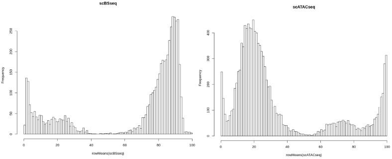

Therefore, we are going to model the scBSseq and scATACseq data as coming from Benoulli distribution. We will further make the scBSseq and scATACseq data sets purely binary by encoding values below 50 as 0 and above 50 as 1 and removing low-variance features to avoid redundancy:

library("mixOmics")

scBSseq <- ifelse(scBSseq < 50, 0, 1)
my_nearZeroVar <- nearZeroVar(as.data.frame(t(scBSseq)))
scBSseq <- scBSseq[-which(rownames(scBSseq) %in% rownames(my_nearZeroVar$Metrics)),]

scATACseq <- ifelse(scATACseq < 50, 0, 1)
my_nearZeroVar <- nearZeroVar(as.data.frame(t(scATACseq)))
scATACseq <- scATACseq[-which(rownames(scATACseq) %in% rownames(my_nearZeroVar$Metrics)),]

Further, we will create the MOFA object and set the model parameters such as Bernoulli distributions for scBSseq and scATACseq, and Gaussian distribution (due to the log-transform) for the scRNAseq OMICs:

library("MOFA")

omics <- list(scRNAseq = scRNAseq, scBSseq = scBSseq, scATACseq = scATACseq)
MOFAobject <- createMOFAobject(omics)
plotDataOverview(MOFAobject)

DataOptions <- getDefaultDataOptions()
ModelOptions <- getDefaultModelOptions(MOFAobject)
mydistr <- c("gaussian", "bernoulli", "bernoulli")
names(mydistr) <- c("scRNAseq", "scBSseq", "scATACseq")
ModelOptions$likelihood <- mydistr
ModelOptions$numFactors <- 20

TrainOptions <- getDefaultTrainOptions()
TrainOptions$seed <- 1234

# Automatically drop factors that explain less than 3% of variance in all omics
TrainOptions$DropFactorThreshold <- 0.03
TrainOptions$tolerance <- 0.1;
TrainOptions$maxiter <- 1000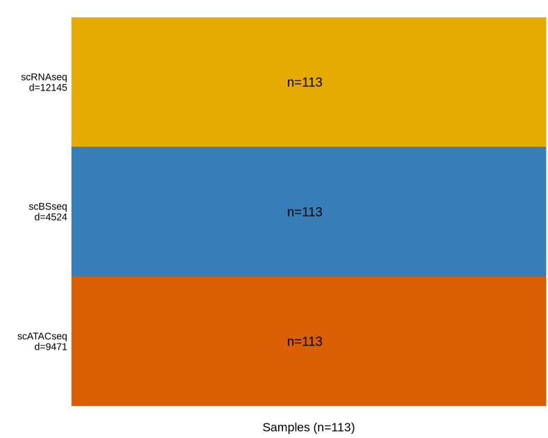

Finally, we are going to prepare the MOFA object and run MOFA. It turns out that MOFA selects only 3 hidden Latent Factors (LFs) that explain more than 3% of variation for the scNMT data set. The main delivery of the MOFa is the great visualization of covariance between the individual OMICs below:

MOFAobject <- prepareMOFA(MOFAobject, DataOptions = DataOptions,
                          ModelOptions = ModelOptions, TrainOptions = TrainOptions)
MOFAobject <- runMOFA(MOFAobject)

r2 <- calculateVarianceExplained(MOFAobject)
plotVarianceExplained(MOFAobject)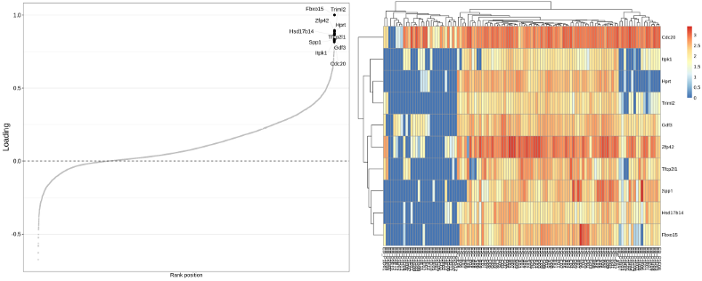

It looks like the loading genes provide a nice separation between ESC and EB cells on the heatmap to the right. Finally, we will display the cells in the low-dimensional latent space, this embedding is the result of integration of the 3 OMICs from the scNMT multi-OMICs data set.

controls <- c("EB_P1D12", "EB_P1E12", "EB_P1F12", "EB_P1G12", "EB_P2B12", "EB_P2D12", "EB_P2E12",
              "EB_P2F12", "EB_P2G12", "ESC_B12", "ESC_C12", "ESC_D12")
colnames(scRNAseq) <- ifelse(colnames(scRNAseq) %in% controls, "CONTROL_CELL", colnames(scRNAseq))
cell_types <- matrix(unlist(strsplit(colnames(scRNAseq), "_")), ncol = 2, byrow = TRUE)[, 1]

plotFactorScatter(MOFAobject, factors = 1:2, color_by = as.factor(cell_types))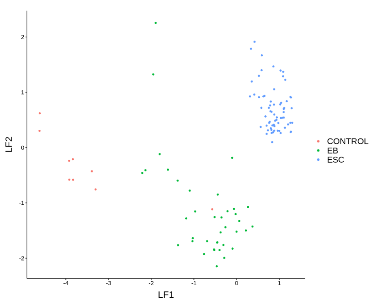

We conclude that MOFA projected the 3 OMICs from scNMT data set into a common latent space where technological differences are omitted and only common variation is taken into account. The integrative approach was able to successfully distinguish between the 3 cell types: ESCs, EBs and Controls.

Summary

In this post, we have learnt that Multi-OMICs Factor Analysis (MOFA) is an elegant Bayesian based algorithm for OMICs integration via extracting the axes of common variation across the modalities. It is particularly useful for data exploration and understanding the interplay between the OMICs. MOFA is insensitive to missing data and allows combining OMICs from different non-Gaussian statistical distributions.