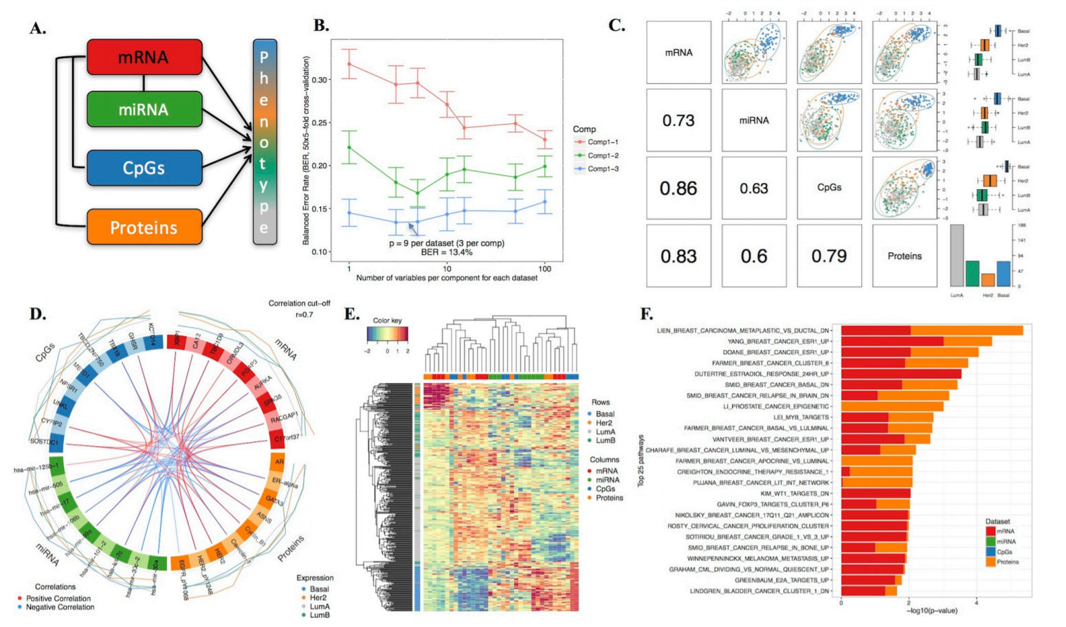
The next few posts will be dedicated to Integrative OMICs analysis which is a modern challenge for computational biology. I will explain basic preprocessing steps to be performed on the data before merging together various types of biological information.

What is Integrative OMICs?

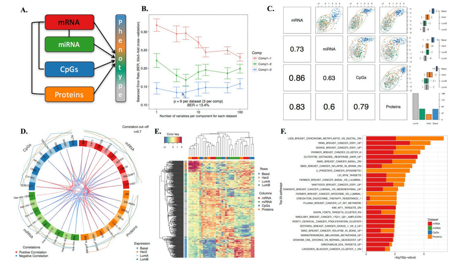
Next Generation Sequencing (NGS) technologies gave rise to manifolds of Biological and Biomedical Big Data such as genomics, proteomics, phenomics, transcriptomics, metabolomics, epigenomics, metagenomics, lipidomics etc., which are often referred to as OMICs due to their common suffix. The rapidly growing amount and diversity of data provides new unique opportunities as well as poses a number of analytical challenges. One challenge is that we assume that the OMICs data should have synergistic effects which allows to more accurately model the behavior of biological cells. In this way, the OMICs integration can identify novel biological pathways that are not necessarily distinguishable in the individual OMICs layers. However, currently there is a lack of mathematical methodologies for performing the OMICs integration although promising workflows such as DIABLO mixOmics are developed.

Why to Select Informative Features?

Another challenge is that combining different types of biological information increases the number of analyzed features while keeping the number of statistical observations (samples) constant. Taking into account that even individual OMICs can be very high-dimensional, their integration is difficult without severe dimensionality reduction or regularization which boils down to selection of most informative features while dropping the noisy ones.

Suppose we are interested in explaining variation in our phenotype of interest, Y, e.g. disease status, and we have a matrix X of explanatory variables (genes) which we assume are responsible for the variation in Y. The question is: do all the explanatory variables in X contribute equally to the variation in Y? Due to lots of noise in biological data it is reasonable to assume that some genes are informative and some are noisy. Since we usually have a limited number of statistical observations we can not afford including noisy genes and have to concentrate on the informative genes, i.e. select features before proceeding with modeling.

For selection we have to test the genes in X against the phenotype Y. However, how should we do it: test all the genes in X together (multivariate feature selection) or one-by-one (univariate feature selection)? Here we are going to compare both ways.

Univariate Feature Selection

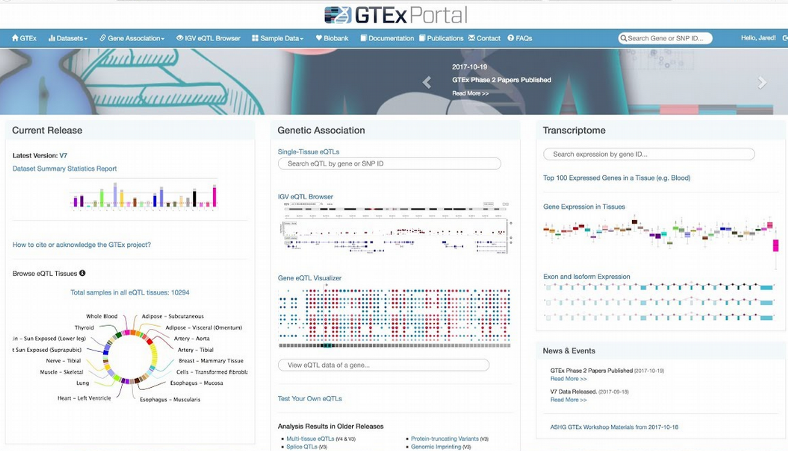
To demonstrate univariate vs. multivariate feature selection I will use RNAseq gene expression data from human skeletal muscles from GTEx Human Tussue Gene Expression Consortium V7. The data set includes n=157 samples and for the sake of simplicity and speed I randomly drew p=1000 genes.

Here we load the gene expression matrix $X$ and remove lowly expressed genes. The phenotype of interest will be Gender, for simplicity. In other words, we are going to find expression of which genes in human skeletal muscles manifests phenotypic differences between 99 Males and 58 Females in our case. Let us visualize the 157 samples of Males and Females via displaying the PCA plot.

library("mixOmics")
X <- read.table("GTEX_SkeletalMuscles_157Samples_1000Genes.txt",
                header = TRUE, row.names = 1, check.names = FALSE, sep = "\t")
X <- X[, colMeans(X) >= 1]
Y <- read.table("GTEX_SkeletalMuscles_157Samples_Gender.txt",
                header = TRUE, sep = "\t")$GENDER
                
pca.gtex <- pca(X, ncomp = 10)
plot(pca.gtex)
plotIndiv(pca.gtex, group = Y, ind.names = FALSE, legend = TRUE,
          title = 'PCA on GTEX Skeletal Muscles')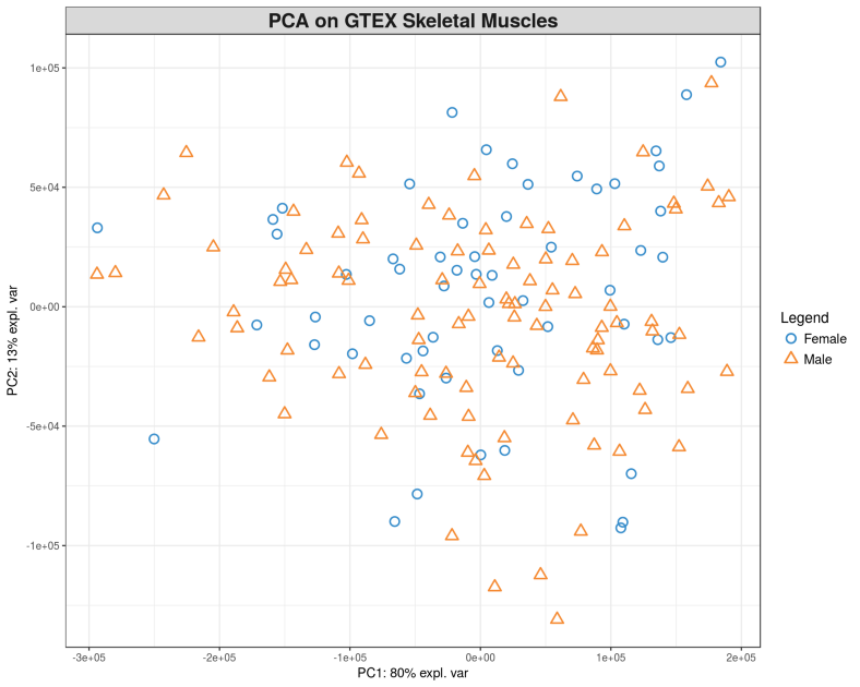

The PCA plot demonstrates a lot of variation between the samples within both $PC_{1}$ and $PC_{2}$, but there is no clear segregation of Males and Females based on their skeletal muscle gene expression data. A way to understand which genes are behind the variation between the samples would be to test the correlation of each individual gene against the Gender, in our case this is equivalent to the Differential Gene Expression (DGE) analysis. Here we will use a simple non-parametric Spearman correlation for inferring relation between $X$ and $Y$, we will test all genes in $X$ one-by-one against $Y$, adjust the p-values of correlations for multiple testing using False Discovery Rate (FDR) and sort genes by FDR.

rho <- vector()
p <- vector()
a <- seq(from = 0, to = dim(X)[2], by = 100)

for (i in 1:dim(X)[2]) {
  corr_output <- cor.test(X[, i], as.numeric(Y), method = "spearman")
  rho <- append(rho, as.numeric(corr_output$estimate))
  p <- append(p, as.numeric(corr_output$p.value))
  if (isTRUE(i %in% a) == TRUE) { print(paste("FINISHED ", i, " FEATURES", sep = ""))
}

output <- data.frame(GENE = colnames(X), SPEARMAN_RHO = rho, PVALUE = p)
output$FDR <- p.adjust(output$PVALUE, method = "fdr")
output <- output[order(output$FDR, output$PVALUE, - output$SPEARMAN_RHO), ]
head(output, 10)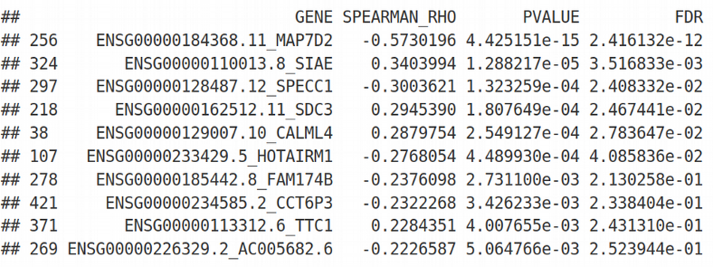

We get the genes ranked by their individual association with Gender and can apply the traditional cutoff FDR=0.05 for selecting informative / significant genes. Next, we can combine those selected genes into a predictive score, this seems like an attractive idea. However, in practice this type of prediction based on univariate feature selection works very poorly because it has two problems:

• Univariate feature selection does not defeat the Curse of Dimensionality issue since FDR correction is not enough for this purpose, i.e. it is prone to overfitting and has a poor generalization.
• Univariate feature selection does not account for multicollinearity between features, i.e. when features are strongly correlated with each other.

The shortcomings mentioned above can be addressed with the Sparse Linear Models, i.e. models with regularization penalties like LASSO / Ridge / Elastic Net, or Partial Least Squares (PLS) regression or discriminant analysis, basic techniques for Multivariate feature selection.

The simplest way to simultaneously account for all explanatory variables in the X matrix would be to put them together into the multiple or multivariate linear model and perform the Ordinary Least Squares (OLS) minimization:

\[ Y = \beta_{1} X_{1} + \beta_{2} X_{2}  + \epsilon \]

\[ OLS = (y -  \beta_{1} X_{1} + \beta_{2} X_{2})^2 \]

Here for simplicity we used only two predictors $X_{1}$ and $X_{2}$, but there can be thousands and millions of them. It implies that in order to minimize the $OLS$ cost function we have to work in high-dimensional space which is inherently difficult because of the Curse of Dimensionality. This leads to a very unstable solution of multiple linear regression. To overcome this obstacle we can add a penalty term to the above $OLS$ cost function:

\[ OLS_{penalized} = (y -  \beta_{1} X_{1} + \beta_{2} X_{2})^2  + \lambda [\alpha (\lvert \beta_{1} \rvert + \lvert \beta_{2} \rvert ) + (1 - \alpha) (\beta_{1}^2 + \beta_{2}^2  ) ] \]

Here, $\lambda$ is called Lagrange multiplier and is a measure of how much penalty we would like to put on our linear model, its optimal value is found through cross-validation. The parameter $\alpha$ is usually fixed, but in principle can also be found through cross-validation, the type of regularization is called:

1. LASSO if \( \alpha=1 \),
2. Ridge if \( \alpha=0 \)
3. Elastic Net if \( \alpha=0.5 \).

These penalty methods have a few differences which are good to remember when you select a method for your analysis. LASSO is the most strict penalty and works best on the data with lots of noise. The problem of LASSO is that it can not fully handle multi-collinearity among predictors. If two variables are strongly correlated, LASSO will select only one of them (by chance) and set the coefficient in front of the other one to zero. Sometimes this type of feature selection can be problematic if it happens that the feature that was ignored / omitted has more physical / biological meaning than the one which was selected by LASSO.

This problem can be avoided with Ridge penalty, in addition Ridge is much more stable for numerical minimization as it provides a fully convex manifold in the high-dimensional space. However, in ultra high-dimensional spaces Ridge can be too permissive and select many noisy features which might not be desirable. Elastic Net penalty provides a compromise between LASSO and Ridge and is generally preferred and recommended by Machine Learning practitioners. Let us use LASSO, perform cross-validation an check which genes were selected:

library("glmnet")

lasso_fit <- cv.glmnet(as.matrix(X), Y, family = "binomial", alpha = 1)
plot(lasso_fit)
coef <- predict(lasso_fit, s = "lambda.min", type = "nonzero")
colnames(X)[unlist(coef)]

result <- data.frame(GENE = names(as.matrix(coef(lasso_fit, s = "lambda.min"))
                                 [as.matrix(coef(lasso_fit, s = "lambda.min"))[, 1] != 0, 1])[-1],
                     SCORE = as.numeric(as.matrix(coef(lasso_fit, s = "lambda.min"))
                                       [as.matrix(coef(lasso_fit, s = "lambda.min"))[, 1] != 0, 1])[-1])
result <- result[order(-abs(result$SCORE)), ]
print(head(result, 10))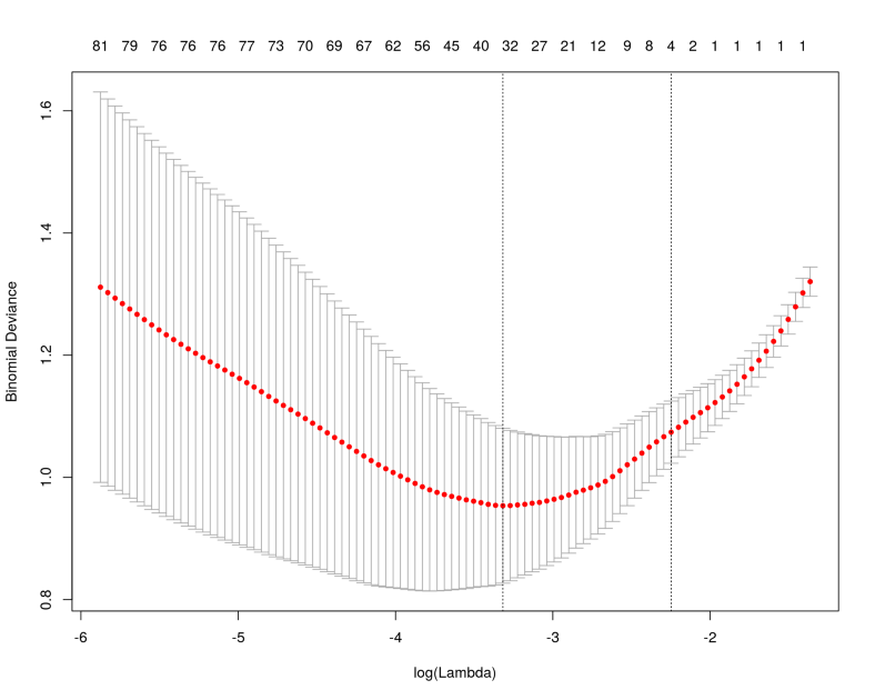

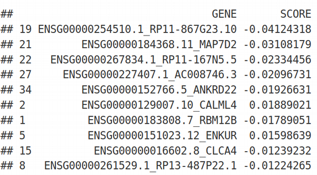
As we can see, LASSO selected approximately 30 features as informative and ranked them by its internal score. The ranking looks quite different compared to the univariate feature selection even though the gene MAP7D2 appears on the top of both feature selection methods.

Another elegant multivariate feature selection technique is the Partial Least Squares (PLS) regression and discriminant analysis which is also called (by its author) Projection on Latent Structures (PLS). The idea behind PLS is that it performs feature selection via maximizing the covariance between $X$ and $Y$:

\[ \max_{\beta} cov(X, Y) => \hat{\beta} \]

Let us perform the PLS discriminant analysis (PLS-DA) on the gene expression matrix X using the gender Y for supervision. It can be thought as multivariate selection of genes that provide largest separation between Males and Females.

library("mixOmics")

gtex.plsda <- plsda(X, Y, ncomp = 2)
background <- background.predict(gtex.plsda, comp.predicted = 2, dist = "max.dist")

plotIndiv(gtex.plsda, comp = 1:2, group = Y, ind.names = FALSE, ellipse = TRUE,
          legend = TRUE, title = 'PLSDA on GTEX Skeletal Muscles', background = background)
          
plotLoadings(gtex.plsda, comp = 1, title = 'Loadings on comp 1', contrib = 'max',
             method = 'median', ndisplay = 10, size.name = 0.6)

plotLoadings(gtex.plsda, comp = 2, title = 'Loadings on comp 2', contrib = 'max',
             method = 'median', ndisplay = 10, size.name = 0.6)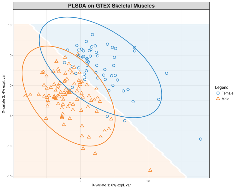

Here we can clearly see the separation between Males and Females, compare this figure with the PCA plot above where we did not see any segregation. To see which genes provide the gender segregation we display the PLS loadings:

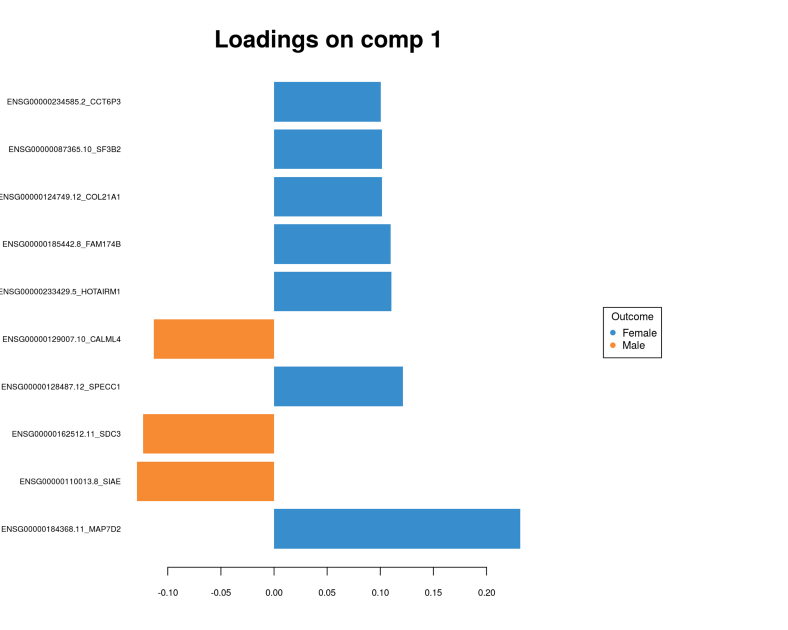
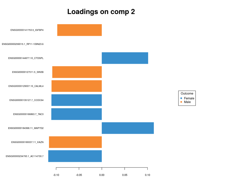
Again, we conclude that the multivariate feature selection via PLS provided a set of genes which looks quite different from the univarite feature selection. Further we are going to use the sets of genes selected in multivariate fashion for integrating different OMICs layers.

Summary

In this article, we have learnt that OMICs integration provides a promising next step for accurate modeling of biological processes. However, a feature pre-selection often has to be done prior to the integration to overcome the Curse of Dimensionality. Univariate feature selection is simple, however it suffers from poor generalizability and does not account for multicollinearity. Multivariate feature selection methods such as LASSO, Ridge, Elastic Net and PLS are preferable for working with high-dimensional biological data.