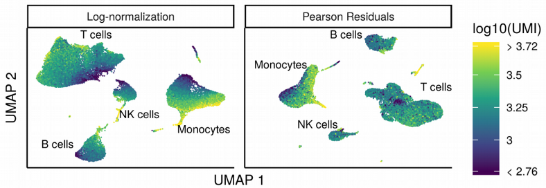
Here we are going to talk about the challenges of removing technical variation in the exciting single cell genomics area by comparing most popular normalization algorithms.

From Bulk to Single Cell Normalization

It is widely recognized that the massive cell-to-cell gene expression variation in the single cell RNA sequencing (scRNAseq) experiments can be to a large extent technical and thus confound the biological variation related to cell types. The sources of technical variation vary from PCR amplification bias to reverse transcription (RT) efficiency and stochasticity of molecular sampling during the preparation and sequencing steps. Therefore normalization across cells has to be applied in order to eliminate the technical variation and keep the biological one. However, common bulk RNAseq methods such as TMM and DESeq are based on constructing per cell size factors which represent ratios where each cell is normalized by a reference cell built by some sort of averaging across all other cells.

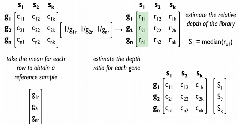
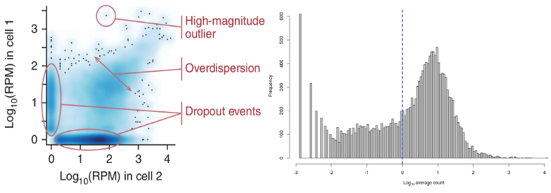
A peculiarity of scRNAseq data is that they contain in contrast to bulk RNAseq large amounts of stochastic zeros owing to low amounts of RNA per cell and imperfect RNA capture efficiency (dropout). Therefore the TMM and DESeq size factors may become unreliably inflated or equal to zero. Therefore new single cell specific normalization methods were developed accounting for the large amounts of zeros in the scRNAseq data.

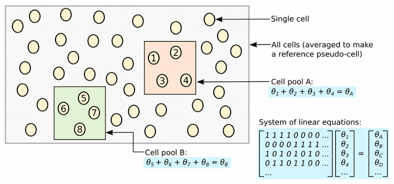
A very elegant attempt of accounting for stochastic zeros in the normalization procedure was made in Marioni’s lab with the deconvolution normalization method. The idea behind the algorithm is to represent all cells by a number of pools of cells, for each pool expression values from multiple cells are summed, which results in fewer zeros, and scaled by an average expression across all cells. Constructed in this way per pool size factors can be deconvolved in a linear system of equations yielding the per cell size factors.

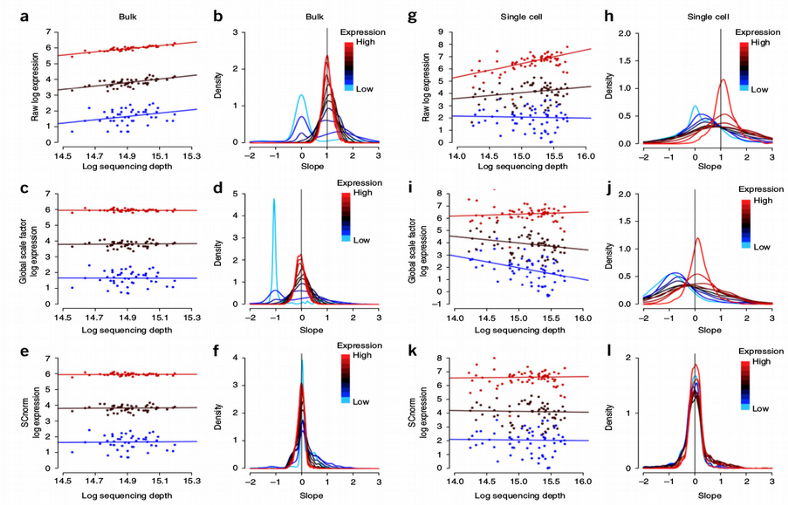
A disadvantage of such a “global size factor approach” is that different groups of genes should not be normalized with the same constant per cell size factor but it should be adjusted individually for each group of genes such as highly, moderately and lowly expressed. This was taken into account in the SCnorm and more recent Pearson residuals normalization algorithms. Both are based on regressing out the sequencing depth bias for different groups of genes.

Below we will compare different popular normalization strategies using the Innate lymphoid cells (ILC) scRNAseq data from Å. Björklund et al., Nature Immunology 17, p. 451–460 (2016)

Comparing scRNAseq Normalization Methods

The scRNAseq analysis workflow is quite complicated, here I will concentrate on the results but encourage you to check the full code examples here.

First of all, the ILC scRNAseq data set was produced with the SmartSeq2 full-length transcript sequencing technology, and includes very handy spike-ins (control transcripts with constant concentration across cells) for assessing the technological background noise. These spike-ins can be used for detecting a set of genes with variation above the noise level via plotting the Coefficient of Variation (CV=sd/mean) as a function of the mean gene expression for each normalization method:

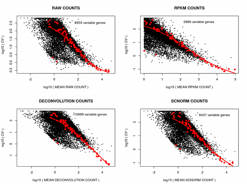
On these plots: one point is one gene, the red curve represents the variation of the spike-ins, the genes above the spike-in curve demonstrate the variation above the technical variation (Highly Variable Genes). One can observe, the number of variable genes varies depending on the normalization method. The RPKMnormalization demonstrates the lowest number of variable genes which is perhaps due to spike-ins short length which is used for normalization in the RPKM. Next, we will examine how the Principal Component Analysis (PCA) plot varies depending on the scRNAseq normalization strategy:

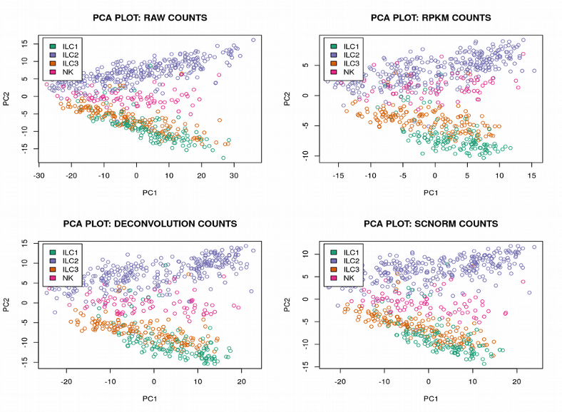
It is hard to see any difference between the normalization methods, the PCA plots look nearly identical demonstrating the cells from the 4 ILC clusters heavily overlapping. Further, as expected, we can get a much more distinct clustering of the ILC cells using the tSNE plots:

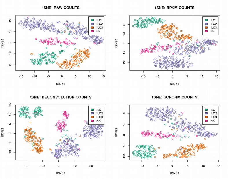
However, the way of normalization does not seem to change much the 4 ILC clusters, they are quite clearly visible regardless of the normalization method. Finally, we can compute the size factors for different normalization strategies and check their correlations:

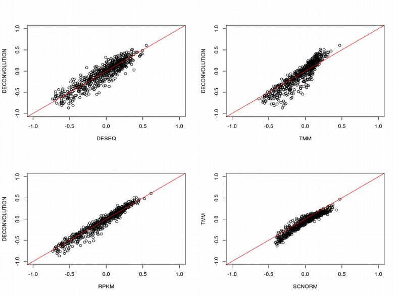
Here for simplicity I averaged the SCnorm size factors across different groups of genes. Surprisingly, the size factors are almost indistinguishable across different normalization methods, even including the bulk RNAseq algorithms TMM and DEseq. However, for other scRNAseq data sets this might not look as good as for ILC.

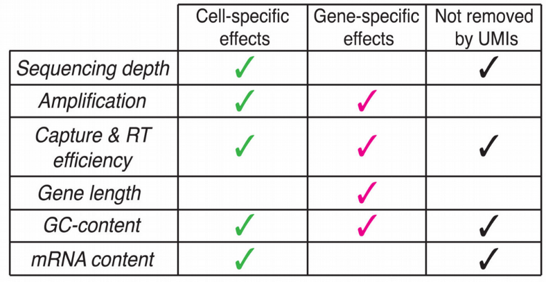
Looking at the plots above, it feels like the importance of normalization for scRNAseq is slightly overestimated as at least for the SmartSeq2 data set the difference in performance was negligible. If cell populations are distinct enough, i.e. if there is a signal in the data, it does not play a major role which scRNAseq normalization method to choose. Moreover, with the widespread use of UMI-based sequencing protocols, the need for complex normalization algorithm becomes even less pronounced as those protocols are in principle capable of removing the amplification and sequencing depth bias as multiple reads are collapsed into a single UMI count.

Summary

In this post, we have learnt that due to massive amounts of stochastic zeros in scRNAseq data sets, the ratio based traditional bulk RNAseq normalization algorithms are not applicable. Deconvolution and SCnorm represent elegant scRNAseq specific normalization methods. However, comparison of scRNAseq normalization methodologies does not demonstrate pronounced difference in their performance, this might become even less notable with the advances in UMI-based scRNAseq protocols.